 R for Spatial Statistics
 Combined Model Plots
The function below will create a model plot that includes the predicted model response, confidence intervals, and the original data points. The function is called with:
- TheModel: A model returned from lm(), glm2(), gam()
- ResponseName: The name of the response variable used to create the model (e.g. "Height", "MaxHt")
- IndepentName: The name of the independent variable to chart the response against. The independent variable must have been used to create TheModel
- TheData: The original data frame used to create the model
- xlab: Optional parameter to replace the ResponseName as the x-axis label
- ylab: Optional parameter to replace the ResponseName as the y-axis label
An example is below.
#########################################################################################
# Creates plots of original data, modeled data, and confidence intervals for one independent
# variable plotted against the response variable for an existing model.
#
# Parameters
# - TheModel - lm, gam, glm, and potentially other models
# - ResponseName - a string containing the name of the response variable used to create the model
# - Independent - a string containing the name of the independent variable used in the creation of the model
# - TheData - Original data used to create the model
# - xlab: Optional parameter to replace the ResponseName as the x-axis label
# - ylab: Optional parameter to replace the ResponseName as the y-axis label
#########################################################################################
CombinedModelPlot=function(TheModel,ResponseName,IndependentName,TheData,xlab="",ylab="")
{
  if (xlab=="") xlab=IndependentName
  if (ylab=="") ylab=ResponseName

  Response=TheData[[ResponseName]]
  Independent=TheData[[IndependentName]]
 # print(Independent)

  # Create a sequence that goes over the entire predictor variable range
  UniformAnnualPrecip = seq(min(Independent), max(Independent), length.out=100)
  NewData=data.frame(IndependentName=UniformAnnualPrecip) # This sets the column name to "IndependentName"
  colnames(NewData) <- c(IndependentName) # set the name of the column to match the name in TheModel

  ThePredictions = predict(TheModel, newdata = NewData,  type="response")
  #response <- predict(TheModel, newdata = data.frame(AnnualPrecip=newx), interval = 'response')
  ThePrediction=predict(TheModel,newdata=TheData,type="response") # create the prediction
  TheStdErr=predict(TheModel,newdata = NewData,se=TRUE) # create the prediction

  #plot(UniformAnnualPrecip,ThePredictions,xlab=xlab,ylab=ylab)

  FinalDataFrame=data.frame(UniformAnnualPrecip,TheStdErr[1],ThePredictions[2])

  # Setup the chart area (jjg - use min/max?)
  plot(Independent,Response,xlab=xlab,ylab=ylab) # Plot the original data

  UpperCI <- ThePredictions + (2 * TheStdErr$se.fit)
  LowerCI <- ThePredictions - (2 * TheStdErr$se.fit)

  # Plot the polygon by going left to right along the top of the polygon
  # and then right to left along the bottom
  polygon(c(UniformAnnualPrecip, rev(UniformAnnualPrecip)), c(UpperCI, rev(LowerCI)), col = 'grey80', border = NA)

  lines(UniformAnnualPrecip, ThePredictions, col = 'black') # plot the response

  # compute the upper and lower confidence intervals
  lines(UniformAnnualPrecip, UpperCI, lty = 'dashed', col = 'black')
  lines(UniformAnnualPrecip, LowerCI, lty = 'dashed', col = 'black')

  # Original points
  points(Independent,Response) # Plot the original data
}
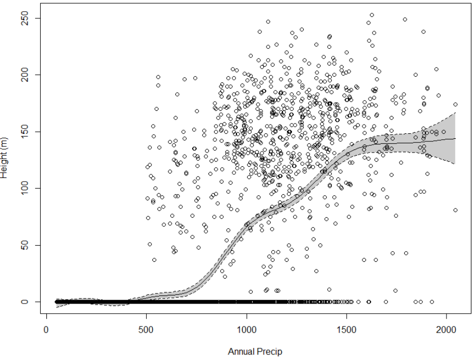
Below is an example of calling the CombinedModelPlot function using a model with "Height" and the response variable and "AnnualPrecip" as the independent variable of interest.
CombinedModelPlot(TheModel,"Height","AnnualPrecip",TheData,xlab="Annual Precip",ylab="Height (m)")